Positive Unlabeled Learning Selected Not At Random
Class proportion estimation without the selected completely at random assumption
Link to Paper|Poster|Source-code
GitHub Link: PULSNAR: Positive Unlabeled Learning Selected Not At Random


Positive and unlabeled (PU) learning is a type of semi-supervised binary classification where the machine learning algorithm differentiates between a set of positive instances (labeled) and a set of both positive and negative instances (unlabeled). PU learning has broad applications in settings where confirmed negatives are unavailable or difficult to obtain, and there is value in discovering positives among the unlabeled (e.g., viable drugs among untested compounds). Most PU learning algorithms make the selected completely at random (SCAR) assumption, namely that positives are selected independently of their features. However, in many real-world applications, such as healthcare, positives are not SCAR (e.g., severe cases are more likely to be diagnosed), leading to a poor estimate of the proportion, α, of positives among unlabeled examples and poor model calibration, resulting in an uncertain decision threshold for selecting positives. PU learning algorithms vary; some estimate only the proportion, α, of positives in the unlabeled set, while others calculate the probability that each specific unlabeled instance is positive, and some can do both. We propose two PU learning algorithms to estimate α, calculate calibrated probabilities for PU instances, and improve classification metrics: i) PULSCAR (positive unlabeled learning selected completely at random), and ii) PULSNAR (positive unlabeled learning selected not at random). PULSNAR employs a divide-and-conquer approach to cluster SNAR positives into subtypes and estimates α for each subtype by applying PULSCAR to positives from each cluster and all unlabeled. In our experiments, PULSNAR outperformed state-of-the-art approaches on both synthetic and real-world benchmark datasets.
PULSCAR algorithm visual intuition.
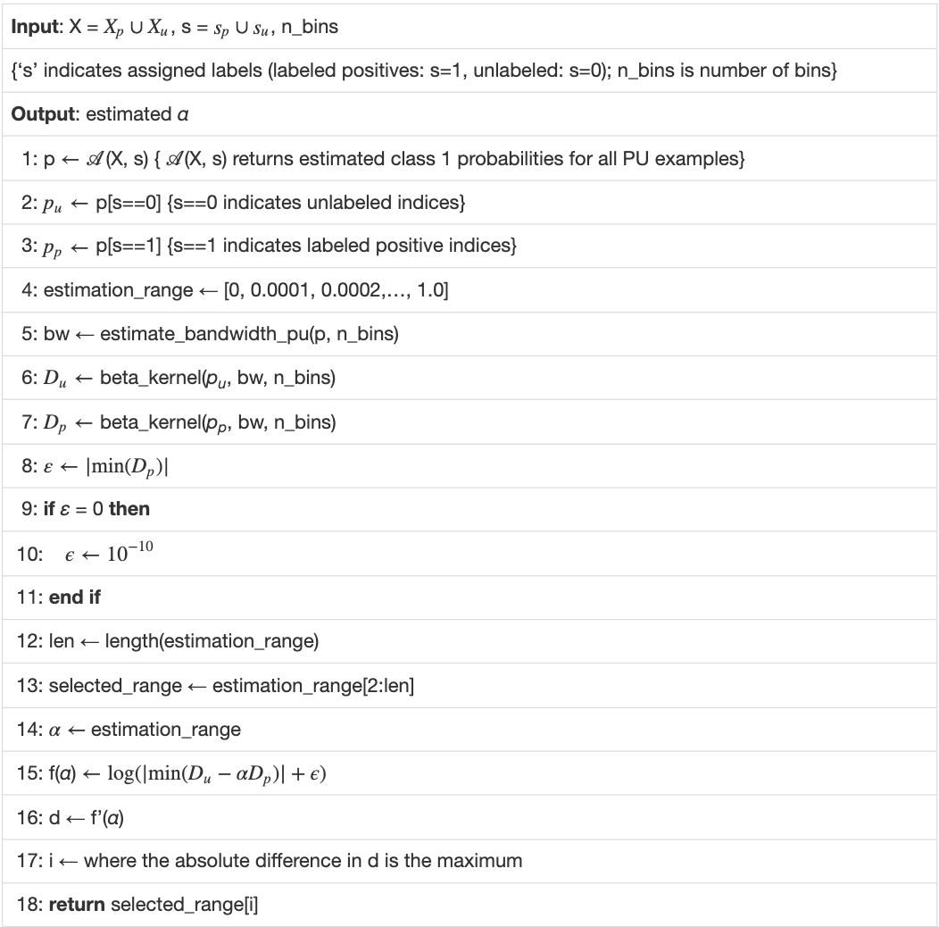
PULSCAR finds the largest αα such that the estimated density of negative examples, Du−αDpDu−αDp, never falls below zero in [0…1]. (A) Probability density estimates for simulated data with α=10%α=10% positive examples in the unlabeled set–estimated density of negative examples (blue) nearly equals the ground truth (green). (B) Overweighting the density of positive examples by α=15%α=15% results in the estimated density of negative examples (blue), dropping below zero. (C) Underweighting the density of positive examples by α=5%α=5% results in the estimated density of negative examples (blue) being higher than the ground truth (green). (D) Estimated α=10.68%α=10.68% selected where the absolute difference in slope of the objective function is largest–very close to ground truth α=10%α=10%. DuDu: PDF of all unlabeled examples (black, dotted); αDpαDp: PDF of unlabeled positive examples scaled by αα (orange, dotdash); Du−αDpDu−αDp: estimated PDF of unlabeled negative examples (blue, solid); (1−α)Dn(1−α)Dn: true PDF of unlabeled negative examples scaled by (1−α)(1−α) (green, twodash).
Schematic of PULSNAR algorithm.
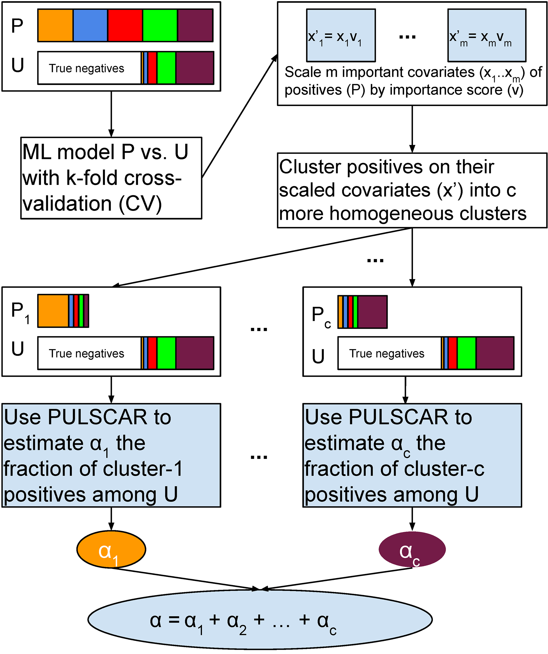
An ML model is trained and tested with five-fold cross-validation (CV) on all positive and unlabeled examples. The important covariates that the model used are scaled by their importance value. Positives are divided into c clusters using the scaled important covariates. c ML models are trained and tested with five-fold CV on the records from a cluster and all unlabeled records. We estimate the proportions ( α1…αcα1…αc) of each subtype of positives in the unlabeled examples using PULSCAR. The sum of those estimates gives the overall fraction of positives in the unlabeled set. P = positive set, U = Unlabeled set.
PULSCAR algorithm.
Our PULSCAR algorithm uses a histogram bin count heuristic to generate a histogram-derived density, then optimizes the beta distribution kernel bandwidth to best fit that density. The approach relies on three key elements: the use of the beta kernel for density estimates, the histogram bin count, and the kernel bandwidth. The beta kernel has important properties, described below, for fitting distributions over the interval [0…1][0…1]. The histogram bin count parameter is set using standard heuristics for fitting a histogram to data, and defines an array of evenly spaced numbers over the interval [0…1][0…1], where the beta kernel density estimates are computed to optimize fitting the histogram. The bandwidth parameter determines the width of the beta kernel, balancing the need for narrower kernels to precisely estimate the distribution with many data points against wider kernels to avoid overfitting when data are sparse. The following three subsections detail these parameters and explain how they are determined.
Suppose both the positive and unlabeled sets contain positives from cc subclasses ( 1…c1…c). With selection bias (SNAR), the subclass proportions will vary between the sets, and thus, the PDF of the labeled positives cannot be scaled by a uniform αα to estimate positives in the unlabeled set. The smallest subclass would drive an αα underestimate with PULSCAR. To address this, we perform clustering on the labeled positives using the key features that differentiate positives from the unlabeled ones. This assumes that these features also correlate with the factors driving selection bias within each subclass. By dividing positives into cc clusters based on these features, we establish that within each cluster, the selection bias is uniformly distributed, implying that all members of a cluster are equally likely to appear in the unlabeled set. Consequently, PU data comprising examples from one cluster and the unlabeled set approximates the SCAR assumption. The uniformity allows for the inference of a cluster-specific αα using PULSCAR, which can be summed over all clusters to provide an overall estimate of positives in the unlabeled set


